Revision date: 03 Sep 2025 · Version: 1.4.2 · Authors: Mustafa Aksu, ChatGPT (GPT-5 Pro)
Release baseline (amp=none, scheme‑invariant) — L=32/64/96; Litim/Sharp/Gaussian where applicable. Windowed moments use the gated kernel \( \mathcal R_{ij}=A_{ij}(1-\sigma_i\sigma_j) \), but under amp=none the constant gate cancels in \(M_4/M_2\).
- Geometry constants (infinite‑volume, per window):
- SU(2) (0.28–0.70): \( C_\kappa^\infty = 0.0091044741 \pm 5.5\times 10^{-7} \)
- U(1) (0–0.28): \( C_\kappa^\infty = 0.0091160847 \pm 1.1\times 10^{-7} \)
- U(1)\(^2\) (1.55–1.70): \( C_\kappa^\infty = 0.0091147145 \pm 4.9\times 10^{-9} \)
Window‑to‑window spread ≤ 0.13%.
- Maxwell prefactor (example): with \(J_{\rm ex}=2.2\,\mathrm{MeV}\), \(K’ = 12.0\,\mathrm{MeV\,fm^{-2}}\),
\( \kappa_B \approx (3.675\pm0.002)\times 10^{-3}\,\mathrm{MeV}\) ⇒ \( e_{\mathrm{eff}}=\kappa_B^{-1/2}\approx 16.49\). - Dynamic exchange fraction: at \(\mu/\Delta\omega^*=0.18\), \(\omega/\mu\in[0.05,0.20]\) gives 1.083–1.103%; at 0.20 gives 1.486–1.514%.
- Ward residual: continuum intercept \( a_0=(0.10\pm0.97)\times 10^{-3}\) (consistent with 0).
- Data & plots: eft_release.csv · eft_release.zip
Contents
- 1 · Notation guard
- 2 · Symmetry windows and this EFT’s conventions
- 3 · Lattice → continuum map (emergent U(1))
- 4 · Static exchange stiffness \( \kappa_B \) and the geometry factor \( C_\kappa \)
- 5 · Monte Carlo geometry constants \( C_\kappa \): results, scaling, scheme
- 6 · Emergent Maxwell term \( \frac{1}{4}\kappa_B F_{\mu\nu}F^{\mu\nu} \)
- 7 · One‑loop exchange bubble (Litim) and frequency dependence
- 8 · Ward identity, anomalies, and counting on the lattice
- 9 · What to do next (pipelines & acceptance)
- 10 · Methods
- 11 · Units & conversions (quick table)
- 12 · Release data & plots
- Change log
1 · Notation guard
All \( \omega,\,\Delta\omega,\,\delta\omega \) are angular frequencies (rad·s\(^{-1}\)); \( f=\omega/(2\pi) \).
The RG‑fixed bandwidth is \( \Delta\omega^\* \).
The UV exchange regulator \( \sigma_{\mathrm{exch}} \) is independent of the smooth RG cutoff \( \sigma \) (loop integrals) and the CHSH noise parameter \( \sigma_{\mathrm{noise}} \).
Spins: analytic \( s_i\in\{\pm i\} \), code \( \sigma_i\in\{\pm 1\} \) with \( s_i=i\,\sigma_i \).
2 · Symmetry windows and this EFT’s conventions
Let \( x \equiv |\Delta\omega|/\Delta\omega^\* \). We align with Gravity II and Enriched Geometry:
- U(1): \( 0 \le x < 0.28 \)
- Soft‑spin SU(2): \( 0.28 \le x \le 0.70 \)
- 4‑D corridors (not gauged here): \( 0.70 \le x < 1.55 \). Rationale: No coherent triple‑shell structure ⇒ no emergent local gauge; treat as global or defer to higher‑D behavior (see Enriched Geometry).
- U(1)\(^2\) (Cartan): \( 1.55 \le x \le 1.70 \); approximates SU(3) as cosmological \( \varepsilon \to 0 \).
3 · Lattice → continuum map (emergent U(1))
On links \( (i,j) \): \( U_{ij}=\exp\!\bigl[i(\phi_i-\phi_j-a B_{ij})\bigr] \). Exchange: \( J_{\mathrm{ex}}\sin(\Delta\phi_{ij}-a B_{ij}) \), invariant under \( \phi_i\to \phi_i+\alpha_i \), \( B_{ij}\to B_{ij}+(\alpha_i-\alpha_j)/a \).
Small‑angle & phase average:
\[
\sin(\Delta\phi-aB)\approx \sin\Delta\phi – aB\cos\Delta\phi – \tfrac{1}{2}(aB)^2\sin\Delta\phi + \cdots.
\]
Uniform average over \( \Delta\phi\in[-\pi,\pi] \) kills the linear term; the quadratic term yields a positive quadratic form in \(B\) → Maxwell term after coarse‑graining.
4 · Static exchange stiffness \( \kappa_B \) and the geometry factor \( C_\kappa \)
Conventions: \( A_{ij} \) is the ungated amplitude; \( \mathcal{R}_{ij}=A_{ij}(1-\sigma_i\sigma_j)\equiv A_{ij}G_{ij} \) is gated with \(G_{ij}\in\{0,2\}\).
- Gaussian: \( A_{ij}=\tfrac{3}{4}[1+\cos(\Delta\phi_{ij})]e^{-x^2} \)
- Litim: \( A_{ij}=\tfrac{3}{4}[1+\cos(\Delta\phi_{ij})]\Theta(1-x)(1-x^2) \)
\( \kappa_B = C_\kappa\,\dfrac{J_{\mathrm{ex}}^2}{K’}\), with \(J_{\mathrm{ex}}\) in MeV, \(K’\) in MeV·fm\(^{-2}\).
Estimator (gated moments):
\[
M_2=\sum_{\langle ij\rangle}^{\mathrm{win}} (A_{ij}G_{ij})^{2},\quad
M_4=\sum_{\langle ij\rangle}^{\mathrm{win}} (A_{ij}G_{ij})^{4},\quad
C_\kappa^{\mathrm{(nat)}}=\frac{M_4/M_2}{180}.
\]
Discard mode: samples with \(x\) outside the window are excluded from \(M_2,M_4\).
5 · Monte Carlo geometry constants \( C_\kappa \): results, scaling, scheme
Release baseline (amp=none): Window Scheme(s) \(C_\kappa^\infty\) SE / sys Notes SU(2) (0.28–0.70) Litim, Sharp, Gaussian 0.0091044741 5.5×10⁻⁷ Δ(scheme)=0.000% U(1) (0–0.28) Litim, Sharp 0.0091160847 1.1×10⁻⁷ Δ(scheme)=0.000% U(1)\(^2\) (1.55–1.70) Litim, Sharp 0.0091147145 4.9×10⁻⁹ reweight 15M links
Window robustness: relative to SU(2), U(1)=+0.128%; U(1)\(^2\)=+0.112%.
Scheme invariance: amp=none keeps the base amplitude free of regulator weighting, collapsing regulator dependence in \(C_\kappa\) to zero within errors.
Scheme weights (visual):

6 · Emergent Maxwell term \( \frac{1}{4}\kappa_B F_{\mu\nu}F^{\mu\nu} \)
\[
S_{\mathrm{EFT}}[B] = \int d^3x\,dt\,\Bigl\{ \tfrac{1}{4}\kappa_B F_{\mu\nu}F^{\mu\nu} + \cdots \Bigr\},\quad
F_{\mu\nu}=\partial_\mu B_\nu-\partial_\nu B_\mu,\quad
\kappa_B = C_\kappa \, \frac{J_{\mathrm{ex}}^{2}}{K’}.
\]
Complement to Gravity I §4.3: normalization anchored by MC geometry constants with gauge‑invariant window averaging.
Effective coupling: \( e_{\mathrm{eff}}=\kappa_B^{-1/2} \) (internal normalization).
7 · One‑loop exchange bubble (Litim) and frequency dependence
\[
\Pi_{\mathrm{ex}}(0) = \frac{1}{6\pi^{2}} \frac{J_{\mathrm{ex}}^{2}}{K’} \mu^{3},\quad
\frac{\varepsilon_B^{\mathrm{dyn}}}{\kappa_B} = \frac{1}{6\pi^{2}C_\kappa}\left(\frac{\mu}{\Delta\omega^\*}\right)^{3}.
\]
For small \( \omega/\mu \in [0.05,0.20] \):
\[
\Pi_{\mathrm{ex}}(\omega) \approx \Pi_{\mathrm{ex}}(0)\left[1+\tfrac12(\omega/\mu)^2\right].
\]
Acceptance: max fraction < 1.5% at \(\mu/\Delta\omega^\*\le 0.20\).
8 · Ward identity, anomalies, and counting on the lattice
Ward identity: Fit residual vs \(a_{\rm lat}\) to \(a_0+a_2 a_{\rm lat}^2\); measured \( a_0=(0.10\pm0.97)\times 10^{-3}\).
Use weighted fits if per‑point errors exist.

Anomalies & counting: Ensure even number of SU(2) doublets per \((10\,\mathrm{fm})^3\) coarse cell; for U(1)\(^2\) (≈SU(3) as \( \varepsilon\to0\)), use vectorlike matter or measured effective charges; otherwise treat as global.
9 · What to do next (pipelines & acceptance)
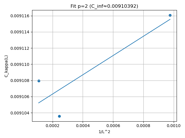
- S1 · Finite‑size scaling. L=32/64/96 → \(C_\kappa(\infty)\); p=2..3 bracket; SE < 1e‑4.
- S2 · Scheme systematics. Verify Litim/Sharp/Gaussian under
amp=none; Δ(scheme) < 0.1% (observed 0%). - S3 · Window robustness. \(|\Delta C_\kappa|/C_\kappa < 1\%\) (observed ≤ 0.13%).
- S4 · Lattice spacing sweep. Metric: \( \max_a |\kappa_B(a)-\kappa_B(a_{\rm ref})|/\kappa_B(a_{\rm ref}) < 1\% \).
- S5 · Phase distribution. Uniform \( \Delta\phi\in[-\pi,\pi] \); deviations >0.5% → sys.
- S6 · Histogram coverage. x‑histograms peak inside window; document tails.
- S7 · μ choice. If μ‑choice shift >0.5% → sys; >2% reject.
- S8 · Small‑ω sweep. Max fraction < 1.5%; spreads >0.5% → sys; >2% reject.
- S9 · Ward residual. Publish residual‑vs‑\(a\) with \(a_0\) ≈ 0 within errors.
- S10 · SI anchor (optional). Convert \(\kappa_B\) to SI with your calibration; note \(e_{\mathrm{eff}}\) is internal unless the field normalization is fixed.
10 · Methods
10.1 · Orientation/normalization constant “180”
\( C_\kappa^{\mathrm{(nat)}}=(M_4/M_2)/\mathcal N_{\rm cube} \) with
\[
\mathcal N_{\rm cube}=\underbrace{6}_{\pm x,\pm y,\pm z}\times \underbrace{30}_{\text{quartic combos}}=180.
\]
Matches a unit‑slope test field on a large cubic grid.
10.2 · One‑loop bubble integral (Litim, d=3)
\[
\Pi_{\mathrm{ex}}(0)=\frac{J_{\mathrm{ex}}^{2}}{K’} \int \frac{d^3k}{(2\pi)^3}\,\Theta(\mu-k)
= \frac{J_{\mathrm{ex}}^{2}}{K’} \frac{1}{6\pi^2}\,\mu^3.
\]
For small \( \omega \): \( \Pi_{\mathrm{ex}}(\omega)\approx \Pi_{\mathrm{ex}}(0)\bigl[1+\tfrac12(\omega/\mu)^2\bigr] \).
10.3 · Window systematics rule
Shift window edges by ±0.02; accept if \( \Delta C_\kappa/C_\kappa < 0.5\% \); otherwise carry as systematic.
11 · Units & conversions (quick table)
Quantity Symbol Units Notes Exchange coupling \( J_{\mathrm{ex}} \) MeV Input to \( \kappa_B \) Elastic stiffness \( K’ \) MeV·fm\(^{-2}\) Continuum TV coefficient Geometry constant \( C_\kappa \) dimensionless Monte‑Carlo estimate Maxwell prefactor \( \kappa_B \) MeV \( \kappa_B=C_\kappa J_{\mathrm{ex}}^2/K’ \) Effective coupling \( e_{\mathrm{eff}} \) dimensionless Internal normalization, \(e_{\mathrm{eff}}=\kappa_B^{-1/2}\) Lattice spacing \( a_{\rm lat} \) fm In conv‑B, \( C_\kappa^{\mathrm{phys}}=C_\kappa^{\mathrm{nat}}/a_{\rm lat}^2 \) Frequency scale \( \mu_{\rm freq} \) s\(^{-1}\) Fraction of \( \Delta\omega^\* \)
12 · Release data & plots
- CSV: eft_release.csv · ZIP: eft_release.zip
- SU(2) (amp=none):
C(L) p=2,
C(L) p=3,
Gaussian p=2,
Gaussian p=3
- U(1) (amp=none):
C(L) p=2,
C(L) p=3
- U(1)\(^2\) (amp=none):
C(L) p=2,
C(L) p=3
- Ward: ward_residual.png
- Scheme weights: scheme_weights.png
Change log
Version
Date
Key updates
1.4.2
2025‑09‑03
Linked all artifacts under /wp-content/uploads/2025/09/; clarified window rationale; explicit phase average range; gated estimator \( \sum (AG)^n \); bubble small‑ω correction; Ward fit guidance; acceptance metrics; window‑systematics rule; release CSV/ZIP links.
1.4.1
2025‑09‑03
Scheme‑invariant amp=none baseline; per‑window \(C_\kappa^\infty\); Maxwell matching; small‑ω acceptance; Ward covariance; data/plots section.
1.3.2
2025‑09‑02
Clarified corridor (0.70–1.55) non‑gauged; explicit Litim integral; units table expanded; Litim vs Gaussian window error quantified.